Landscape Ecology and Conservation

Authors: Cristina Banks-Leite, David Orme & Flavia Bellotto-Trigo

In this practical, we are going to use R to:

1. obtain landscape metrics from a map;

2. obtain community metrics from a bird dataset; and

3. analyse the data to assess how Atlantic Forest birds are impacted by habitat loss and fragmentation.

Class group exercise

Everyone in the class will have access to the same data but each group will be assigned a specific question that needs to be answered by the Friday sessions of this week. Instructions for this exercise will be in boxes like this one.

On Friday, one representative from each group (make sure to decide this beforehand), will present their results on a single slide. A discussion will follow.

Data exploration exercises

In addition to the instructions for the class exercises, there are some individual exercises, which ask you to explore the data and techniques used. These will be in boxes like this one.

Requirements

We will need to load the following packages. Remember to read this guide on setting up packages on your computer if you are running these practicals on your own machine, not Posit Cloud.

library(terra)
library(sf)
library(landscapemetrics)
library(vegan)
library(ggplot2)

Data sets

The first step is to load and explore the datasets.

Species data

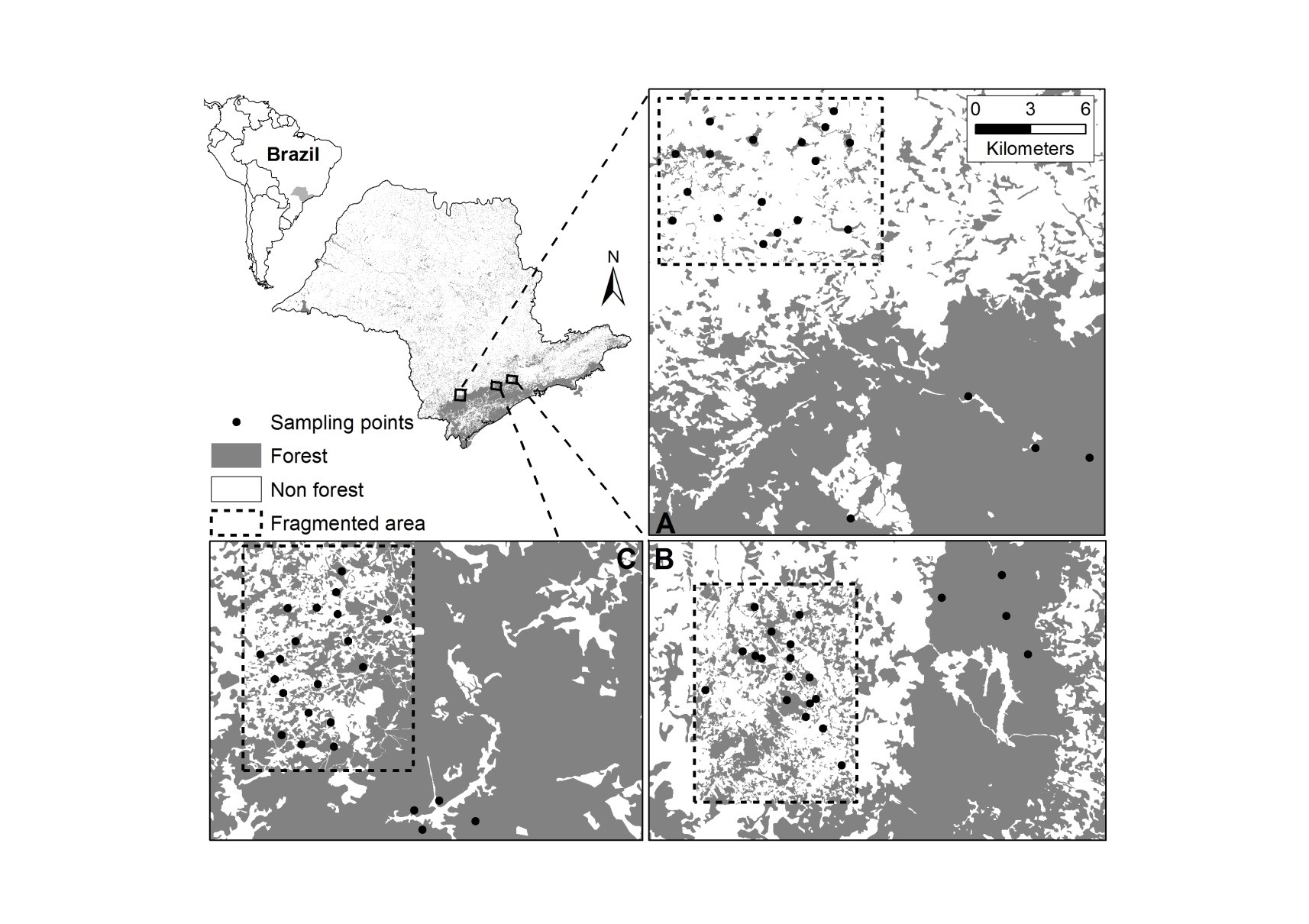
This is a bird data set that was collected in the Brazilian Atlantic Forest between 2001 and 2007. The data set contains the abundance of 140 species that were captured in 65 sites, from three different regions, each containing a control landscape and a 10,000 ha fragmented landscape. The fragmented landscapes varied in their proportions of forest cover (10, 30 and 50% cover).

More info about the data set can be found in the following papers:

• Banks-Leite, C., Ewers, R. M., & Metzger, J. P. (2012). Unraveling the drivers of community dissimilarity and species extinction in fragmented landscapes. Ecology 93(12), 2560-2569. https://esajournals.onlinelibrary.wiley.com/doi/10.1890/11-2054.1

• Banks-Leite, C., Ewers, R. M., Kapos, V., Martensen, A. C., & Metzger, J. P. (2011). Comparing species and measures of landscape structure as indicators of conservation importance. Journal of Applied Ecology 48(3), 706-714. https://doi.org/10.1111/j.1365-2664.2011.01966.x

There are two files to load.

Sites data

First, we can load the sites data and use the longitude and latitude coordinates (WGS84, EPSG code 4326) to turn the data into an sf object.

sites <- read.csv("data/brazil/sites.csv", header = TRUE)
sites <- st_as_sf(sites, coords=c('Lon','Lat'), crs=4326)
plot(sites[c('Landscape_ID')], key.pos=4, axes=TRUE)
str(sites)

Classes ‘sf’ and 'data.frame':	65 obs. of  5 variables:
 $ Site        : chr  "Alce" "Alcides" "Alteres" "Antenor" ...
 $ Landscape   : chr  "Fragmented" "Fragmented" "Fragmented" "Fragmented" ...
 $ Percent     : int  50 30 10 50 90 50 30 50 10 10 ...
 $ Landscape_ID: chr  "B" "C" "A" "B" ...
 $ geometry    :sfc_POINT of length 65; first list element:  'XY' num  -47.5 -23.9
 - attr(*, "sf_column")= chr "geometry"
 - attr(*, "agr")= Factor w/ 3 levels "constant","aggregate",..: NA NA NA NA
  ..- attr(*, "names")= chr [1:4] "Site" "Landscape" "Percent" "Landscape_ID"

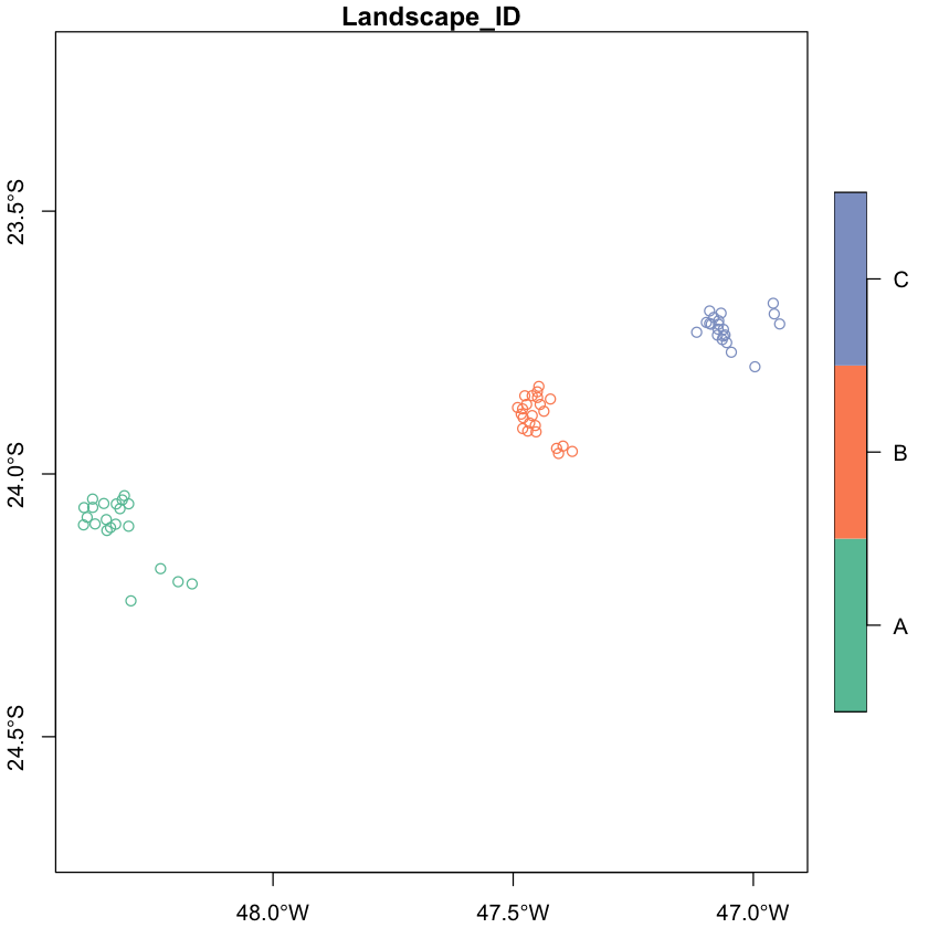
Region A corresponds to the fragmented landscape with 10% forest cover (and adjcent control), region B corresponds to fragmented landscape with 50% of cover (and control) and region C corresponds to fragmented landscape with 30% of cover (and control). The sites data set describes the characteristics of the sampling sites:

• Landscape: whether the site belong to a fragmented or a continuously-forested control landscape,

• Percent: the proportion of forest cover at the 10,000 ha landscape scale, and

• Landscape_ID: as we just saw, fragmented landscapes were paired with a control landscape, so this variable gives you the information of which sites belonged to the same region.

Abundance data

Next, read in the data set showing the sites x species abundance matrix. As you’ll see, a lot of the species were only caught once or twice and there are lots of 0s in the matrix. Few species are globally common.

# Load the abundance data and use the first column (site names) as row names
abundance <- read.csv("data/brazil/abundance.csv", row.names=1, stringsAsFactors = FALSE)
dim(abundance)

1. 65
2. 140

The abundance data has 65 rows - one for each site - and there are 140 species that were seen in at least one site.

Data checking

It is always worth looking at the data frames in detail, to understand their contents. We have used str to look at the structure but you can also use View to look at the dataset as a table.

View(sites)
View(abundance)

It is also wise to check for missing data. Some key tools:

summary(abundance) # NAs will be counted if found
any(is.na(abundance))

Landcover data

We will calculate the landscape metrics from a landcover map for the study region. If you want to know more about the origin of the map, check https://mapbiomas.org. It is in Portuguese but Google should translate it for you! This is a database of land cover through time for the entire country of Brazil - we are using data contemporary with the bird sampling.

The map is a GEOTIFF file of landcover classes, therefore we are going to use the function terra::rast function to load the map. First, load the map and check its coordinate system:

# load map
landcover <- rast("data/brazil/map.tif")
print(landcover)

class       : SpatRaster 
dimensions  : 7421, 11132, 1  (nrow, ncol, nlyr)
resolution  : 0.0002694946, 0.0002694946  (x, y)
extent      : -49.00004, -46.00003, -24.99993, -23.00002  (xmin, xmax, ymin, ymax)
coord. ref. : lon/lat WGS 84 (EPSG:4326) 
source      : map.tif 
name        : map 
min value   :   0 
max value   :  33 

The map has 33 values for the 33 different landcover classes including: forest, plantation, mangroves, etc. We will only be looking at forests (landcover class 3).

Another important thing is that the map is quite large and has a very fine resolution (0.000269° is about 1 arcsecond or ~30 metres). There are over 82 million pixels in the image and so the data is slow to handle. In fact, although the file loaded quickly, it did not load the actual data. The terra package often does this to keep the memory load low - it only loads data when requested and has tricks for only loading the data it needs. You can see this:

inMemory(landcover)

FALSE

We’re not even going to try and plot this map! This is something that would be much easier to view in QGIS, which handles visualising big data well. We will extract some data from it in the next section.

Calculating landscape metrics

Landscape data processing

Before we calculate landscape metrics, we first need to process the land cover data to make it easier to work with. In particular, using the whole map is very computationally demanding so we need to reduce the data down to the scale of the focal regions to extract landscape metrics for each site. In order to do that we need to:

1. Identify a smaller region of interest for the sites

2. Crop the landcover raster down to this region, to use a small dataset.

3. Convert the landcover to a binary forest - matrix map.

4. Reproject the data into a suitable projected coordinate system.

# Get the bounding box and convert to a polygon
sites_region <- st_as_sfc(st_bbox(sites))

# Buffer the region by 0.1 degrees to get coverage around the landscape.
# This is roughly 10 kilometres which is a wide enough border to allow
# us to test the scale of effects.
sites_region <- st_buffer(sites_region, 0.1)

# Crop the landcover data and convert to a binary forest map
sites_landcover <- crop(landcover, sites_region)
sites_forest <- sites_landcover == 3
print(sites_forest)

class       : SpatRaster 
dimensions  : 2188, 5407, 1  (nrow, ncol, nlyr)
resolution  : 0.0002694946, 0.0002694946  (x, y)
extent      : -48.3988, -46.94164, -24.25424, -23.66459  (xmin, xmax, ymin, ymax)
coord. ref. : lon/lat WGS 84 (EPSG:4326) 
source(s)   : memory
varname     : map 
name        :   map 
min value   : FALSE 
max value   :  TRUE 

If you check that final output, you will see that the values changed to values: 0, 1 (min, max).

Now that we have the regional forest for the sites, we can reproject the data. We will use UTM Zone 23S (EPSG: 32723) for all of the landscapes. Remember that the landcover class data is categorical - we have to use method='near' when projecting the data. We’ve also set a resolution of 30 metres.

sites_utm23S <- st_transform(sites, 32723)
# This takes a little while to run!
sites_forest_utm23S <- project(sites_forest, "epsg:32723", res=30, method='near')

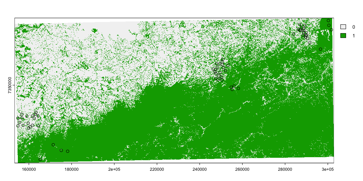
Just to check, we should now be able to plot the sites and forest.

plot(sites_forest_utm23S)
plot(st_geometry(sites_utm23S), add=TRUE)

Extracting landscape metrics

You can now explore the functions in the package landscapemetrics to measure different landscape metrics. You can also look at the complete set of 132 landscape metrics that the package will calculate:

lsm_abbreviations_names

A tibble: 133 × 5

metric	name	type	level	function_name
<chr>	<chr>	<chr>	<chr>	<chr>
area	patch area	area and edge metric	patch	lsm_p_area
cai	core area index	core area metric	patch	lsm_p_cai
circle	related circumscribing circle	shape metric	patch	lsm_p_circle
contig	contiguity index	shape metric	patch	lsm_p_contig
core	core area	core area metric	patch	lsm_p_core
enn	euclidean nearest neighbor distance	aggregation metric	patch	lsm_p_enn
frac	fractal dimension index	shape metric	patch	lsm_p_frac
gyrate	radius of gyration	area and edge metric	patch	lsm_p_gyrate
ncore	number of core areas	core area metric	patch	lsm_p_ncore
para	perimeter-area ratio	shape metric	patch	lsm_p_para
perim	patch perimeter	area and edge metric	patch	lsm_p_perim
shape	shape index	shape metric	patch	lsm_p_shape
ai	aggregation index	aggregation metric	class	lsm_c_ai
area_cv	patch area	area and edge metric	class	lsm_c_area_cv
area_mn	patch area	area and edge metric	class	lsm_c_area_mn
area_sd	patch area	area and edge metric	class	lsm_c_area_sd
ca	total (class) area	area and edge metric	class	lsm_c_ca
cai_cv	core area index	core area metric	class	lsm_c_cai_cv
cai_mn	core area index	core area metric	class	lsm_c_cai_mn
cai_sd	core area index	core area metric	class	lsm_c_cai_sd
circle_cv	related circumscribing circle	shape metric	class	lsm_c_circle_cv
circle_mn	related circumscribing circle	shape metric	class	lsm_c_circle_mn
circle_sd	related circumscribing circle	shape metric	class	lsm_c_circle_sd
clumpy	clumpiness index	aggregation metric	class	lsm_c_clumpy
cohesion	patch cohesion index	aggregation metric	class	lsm_c_cohesion
contig_cv	contiguity index	shape metric	class	lsm_c_contig_cv
contig_mn	contiguity index	shape metric	class	lsm_c_contig_mn
contig_sd	contiguity index	shape metric	class	lsm_c_contig_sd
core_cv	core area	core area metric	class	lsm_c_core_cv
core_mn	core area	core area metric	class	lsm_c_core_mn
⋮	⋮	⋮	⋮	⋮
joinent	joint entropy	complexity metric	landscape	lsm_l_joinent
lpi	largest patch index	area and edge metric	landscape	lsm_l_lpi
lsi	landscape shape index	aggregation metric	landscape	lsm_l_lsi
mesh	effective mesh size	aggregation metric	landscape	lsm_l_mesh
msidi	modified simpson's diversity index	diversity metric	landscape	lsm_l_msidi
msiei	modified simpson's evenness index	diversity metric	landscape	lsm_l_msiei
mutinf	mutual information	complexity metric	landscape	lsm_l_mutinf
ndca	number of disjunct core areas	core area metric	landscape	lsm_l_ndca
np	number of patches	aggregation metric	landscape	lsm_l_np
pafrac	perimeter-area fractal dimension	shape metric	landscape	lsm_l_pafrac
para_cv	perimeter-area ratio	shape metric	landscape	lsm_l_para_cv
para_mn	perimeter-area ratio	shape metric	landscape	lsm_l_para_mn
para_sd	perimeter-area ratio	shape metric	landscape	lsm_l_para_sd
pd	patch density	aggregation metric	landscape	lsm_l_pd
pladj	percentage of like adjacencies	aggregation metric	landscape	lsm_l_pladj
pr	patch richness	diversity metric	landscape	lsm_l_pr
prd	patch richness density	diversity metric	landscape	lsm_l_prd
relmutinf	relative mutual information	complexity metric	landscape	lsm_l_relmutinf
rpr	relative patch richness	diversity metric	landscape	lsm_l_rpr
shape_cv	shape index	shape metric	landscape	lsm_l_shape_cv
shape_mn	shape index	shape metric	landscape	lsm_l_shape_mn
shape_sd	shape index	shape metric	landscape	lsm_l_shape_sd
shdi	shannon's diversity index	diversity metric	landscape	lsm_l_shdi
shei	shannon's evenness index	diversity metric	landscape	lsm_l_shei
sidi	simpson's diversity index	diversity metric	landscape	lsm_l_sidi
siei	simspon's evenness index	diversity metric	landscape	lsm_l_siei
split	splitting index	aggregation metric	landscape	lsm_l_split
ta	total area	area and edge metric	landscape	lsm_l_ta
tca	total core area	core area metric	landscape	lsm_l_tca
te	total edge	area and edge metric	landscape	lsm_l_te

Landscape levels

There are three core levels of calculation and it is important to understand how these are applied within a local landscape:

• The patch level metrics are things that are calculated for every single patch in the local landscape. So in the output, there is one row for each patch and it is identified with a patch id and a class id.

• The class level metrics are aggregated across all patches of a specific class, so there is a row for each class that appears in the local landscape, labelled with a class id (but no patch).

• The landscape metrics aggregate all patches, so there is just one row per landscape.

To show how these values are reported - and how we can use them - the following code uses the sample_lsm function to calculate a set of metrics for patch counts and areas at all three levels, along with the proportion landcover of each class. The local landscape is defined as a circle with a radius of 600 meters. We will use the Alce site as an example:

# Calculate patch areas at patch, class and landscape scale.
lsm <- sample_lsm(sites_forest_utm23S, sites_utm23S, 
                  shape = "circle", size = 600, 
                  plot_id = sites_utm23S$Site, 
                  what = c('lsm_p_area',
                           'lsm_c_np', 'lsm_l_np', 
                           'lsm_c_area_mn', 'lsm_l_area_mn',
                           'lsm_c_pland'))

# Use Alce as an example
alce <- subset(lsm, plot_id=='Alce')
print(alce, n=23)

Warning message:
“The 'perecentage_inside' is below 90% for at least one buffer.”

Warning message:
“[mask] CRS do not match”

# A tibble: 21 × 8
   layer level     class    id metric  value plot_id percentage_inside
   <int> <chr>     <int> <int> <chr>   <dbl> <chr>               <dbl>
 1     1 class         0    NA area_mn 40.1  Alce                 105.
 2     1 class         1    NA area_mn  3.53 Alce                 105.
 3     1 class         0    NA np       2    Alce                 105.
 4     1 class         1    NA np      11    Alce                 105.
 5     1 class         0    NA pland   67.3  Alce                 105.
 6     1 class         1    NA pland   32.7  Alce                 105.
 7     1 landscape    NA    NA area_mn  9.16 Alce                 105.
 8     1 landscape    NA    NA np      13    Alce                 105.
 9     1 patch         0     1 area    78.9  Alce                 105.
10     1 patch         0     2 area     1.26 Alce                 105.
11     1 patch         1     3 area     0.99 Alce                 105.
12     1 patch         1     4 area    28.6  Alce                 105.
13     1 patch         1     5 area     0.72 Alce                 105.
14     1 patch         1     6 area     0.36 Alce                 105.
15     1 patch         1     7 area     2.16 Alce                 105.
16     1 patch         1     8 area     2.07 Alce                 105.
17     1 patch         1     9 area     0.54 Alce                 105.
18     1 patch         1    10 area     1.35 Alce                 105.
19     1 patch         1    11 area     1.17 Alce                 105.
20     1 patch         1    12 area     0.09 Alce                 105.
21     1 patch         1    13 area     0.81 Alce                 105.

# Calculate total area
sum(alce$value[alce$metric == 'area'])

119.07

From that table, you can see that there are 15 patches in the Alce local landscape that sum to 113.13 hectares. That is not quite the precise area of the circular landscape (\(\pi \times 600^2 = 1130973 m^2 \approx 113.1 ha\)) because the landscape is used to select a set of whole pixels rather than a precise circle. The class metrics summarise the areas of the patches by class (11 forest patches, 4 matrix patches) and the landscape metrics aggregate everything. We can use the table to calculate the lsm_l_area_mn value by hand:

# Weighted average of class patch sizes (with some rounding error)
(19.0 * 4 + 3.38 * 11) / 15

7.54533333333333

Merging landscape metrics onto sites

The contents of lsm is rather unhelpful in two ways:

1. The variables are not in separate columns, but stacked in the value and metric fields.

2. Class variables include rows for both the matrix and forest, and we are primarily interested in the forest class metrics.

So, we need a couple of tools to help convert this output into something easier to use:

1. We can use subset to keep just the columns and rows we actually want: forest class metrics and values.

2. We need to reshape the data frame to have a column for each measure. (The help and syntax of the reshape function is notoriously unhelpful - there are other, better tools but this simple recipe works here).

3. Along the way, we should make sure that our variable names are clear - we want the method of calculation of each value to be obvious.

# Drop the patch data and landscape rows
lsm_forest <- subset(lsm, level == 'class')
# Drop down to the forest class and also reduce to the three core fields
lsm_forest <- subset(lsm_forest, class == 1, select=c(metric, value, plot_id))

# Rename the value field so that - when combined with the metric
# name - the local landscape details are recorded
names(lsm_forest)[2] <- 'C600'

# Reshape that dataset so that each metric has its own column
lsm_forest <- reshape(data.frame(lsm_forest), direction='wide', 
                      timevar='metric', idvar='plot_id')
head(lsm_forest, n=10)

A data.frame: 10 × 4

	plot_id	C600.area_mn	C600.np	C600.pland
	<chr>	<dbl>	<dbl>	<dbl>
1	Alce	3.534545	11	32.65306
4	Alcides	4.833000	10	40.46722
7	Alteres	29.070000	1	24.34062
10	Antenor	101.070000	1	84.81873
13	Areial	118.800000	1	100.00000
16	Baleia	10.095000	6	50.90772
19	BetoJamil	5.793750	8	38.80934
22	Bicudinho	11.767500	4	39.56127
25	Boiadeiro	4.680000	4	15.68627
28	Bojado	15.480000	3	38.97281

Now it is easy to match those landscape metrics to the sites data.

sites <- merge(sites, lsm_forest, by.x='Site', by.y='plot_id')

Group exercise

This exercise will consist of obtaining a number of landscape metrics for each of our 65 sites, so we can later use them as explanatory variables in a model to understand how birds are affected by habitat loss and fragmentation.

Each group will focus on a set of metrics that capture different aspects of landscape structure. Look up and read the information for your metrics, so you can have a better understanding of what they mean, and collate them all to the sites.csv spreadsheet (or you can create another spreadsheet). You may need to defend your choice of landscape metric on the presentation!

In all cases, we are interested in the forest specific values of the class metrics, so you will need to subset and reshape the data as above. There is a help page for each metric: for example, ?lsm_c_area_cv.

• Groups SP01, SP02, SP03: Patch size & number of patches

  • Coefficient of variation of patch area (lsm_c_area_cv)

  • Mean of patch area (lsm_c_area_mn)

  • Number of patches (lsm_c_np)

• Groups SP04, SP05, SP06: Connectivity

  • Patch density (lsm_c_pd)

  • Coefficient of variation of euclidean nearest-neighbor distance (lsm_c_enn_cv)

  • Aggregation index (lsm_c_ai)

• Groups SP07, SP08, SP09: Edge effects

  • Coefficient of variation perimeter-area ratio (lsm_c_para_cv)

  • Coefficient of variation of related circumscribing circle (lsm_c_circle_cv)

  • Edge density (lsm_c_ed)

• Groups SP13, SP14: Forest cover

  • There is only one way to measure habitat cover: lsm_c_pland. These groups will also focus on exploring the scale of effect: the spatial scale at which responses are strongest. You’ll need to calculate forest cover using radii of 300, 500, 800, 1100 and 1400 m. Note that lsm_c_pland is a proportion of the area, so does not need to be adjusted for the changing landscape area.

Calculating biodiversity metrics

The over-riding research question we are looking at is:

Is the structure of the bird community influenced by the spatial characteristics of the sites?

However there are lots of different ways of measuring community structure. We will look at measures of overall diversity, community composition and functional diversity.

Measuring site abundance, species richness, species diversity and evenness

Abundance can be measured at the species level, but here we are interested in total community abundance, so the total number of individuals captured at each site. We can only measure bird abundance because this study used mist nets, where each individual was uniquely tagged.

To measure species richness you can use the function specnumber from the vegan package. As we saw in the lecture, Measuring Biodiversity, sometimes you may need to control for sampling effort or number of individuals to compare species richness across sites. You can use rarefaction (with function rarefy) to estimate how many species you would have seen if you had lower sampling effort or fewer individuals. If you’re interested in understanding how species diversity changes, you can measure the Shannon index (\(H\)) by using the function diversity. The vegan package doesn’t have any functions for measuring evenness, but Pielou’s Evenness (\(J\)) is easily measured with the formula below:

# First, we sort the rows of abundance to make sure that they are in the
# same order as the sites data frame.
site_order <- match(rownames(abundance), sites$Site)
abundance <- abundance[site_order, ]

# Now we can store diversity metrics values in the sites data frame
sites$total_abundance <- rowSums(abundance)
sites$richness <- specnumber(abundance)
sites$Srar <- rarefy(abundance, min(sites$total_abundance))
sites$H <- diversity(abundance, index='shannon')
# Pielou's evenness
sites$J <- sites$H / log(sites$richness)

Exploring the data

What is the correlation between richness, diversity, evenness and abundance across sites? You can use the function cor() and plot() the results to better understand the patterns. Which biodiversity metrics would you choose to report your results and why?

# Some example code to modify:
cor(sites$richness, sites$total_abundance)

0.645164054185018

plot(richness ~ total_abundance, data=sites)

Hint: There is no right or wrong answer here. You can choose any metric as long as you understand its advantages and disadvantages.

Species abundance distribution

We could also look at the rank abundance of species to understand if our community is dominated by a few species or to assess the prevalence of rare species. Rare species are those that were caught a few times only. This is very arbitrary and likely to be biased by how easily species are disturbed and trapped.

# Get the total abundance of each _species_
species_abund <- colSums(abundance)
# Transform into relative percent abundance
species_abund_perc <- species_abund / sum(species_abund) * 100
# Plot from most to least abundant
plot(sort(species_abund_perc, decreasing = TRUE))

How does this compare to slide 11 of Measuring Biodiversity lecture which shows the patterns of Amazonian trees and bats? Try doing this for each fragmented landscape to see if trends are affected by habitat cover.

Measuring community composition

Community composition is a class of biodiversity measure that incorporates information on species richness, abundance and species identity. That inclusivity makes them a very informative biodiversity metric but they are also complex to compute and interpret.

There are three stages to assessing community composition:

1. The raw data for community composition is a site by species matrix showing the abundance (or presence) of each species at each site. It is common to transform the site by species data in one or more ways to adjust the emphasis given to the different species before assessing composition.

2. The site by species matrix is then transformed into a dissimilarity matrix - a site by site matrix that quantifies the differences between the communities at each pair of sites.

3. The dissimilarity matrix represents a complex pattern of community differences and an ordination can then be used to identify independent axes of community variation across sites.

All of these steps have multiple options!

Transforming site by species data

There are several common approaches used for transforming site by species matrices before calculating dissimilarities. All of these approaches alter the weighting given to the different species.

1. Reducing abundance data to a binary presence-absence data. This transformation emphasizes differences in species identity and differences in rare species between sites, often giving measures of \(\beta\) diversity, and is also often used when sampling is not thought to give reliable abundance data. The vegdist function (see below) has the option (binary=TRUE) to do this automatically.

2. Scaling abundance data. Variation in the abundance data can be driven by a few common species, particularly when the variation in abundance of some species is much larger than others (e.g. one species varies in abundance from 0 to 1000, and all other species vary from 0 to 10). In our case, the most abundant species only varied from 0 to 24 individuals, so scaling this dataset should not particularly affect the results. Scaling a dataset alters the balance of the analysis to equally weight each species when calculating dissimilarity which can provide more biologically meaningful results.

3. Although this seems counterintuitive, the detectability and distribution of rare species can confound community patterns among the common species. Removing rare species can therefore help make major compositional shifts more obvious. This is particularly important in microbiome studies with thousands of OTUs (e.g. it is common in these studies to exclude the 5% least common OTUs).

We will revisit this but for the moment we will stick with the raw abundance data.

Calculating dissimilarity Indices

Dissimilarity indices are used to compare two sites using the total number (or abundances) of species in each site (A + B), along with the number (or abundances) of species shared between the site (J). These can be calculated using the vegdist function in vegan. A large number of indices have been proposed and can be calculated in vegan: look at the help for both ?vegdist and ?designdist for the details!

We have many options but we have to start somewhere: we will use the Bray-Curtis dissimilarity index computed from raw abundances.

bray  <- vegdist(abundance, method="bray", binary=FALSE)

Have a look at the association matrix (print(bray)), and notice it is triangular. Why do you think that is? We can visualise this data to help understand what is going on. We’re actually going to cheat a bit here - we have a big matrix and the terra package is really good at plotting those quickly…

bray_r <- rast(as.matrix(bray))
plot(bray_r, col=hcl.colors(20))

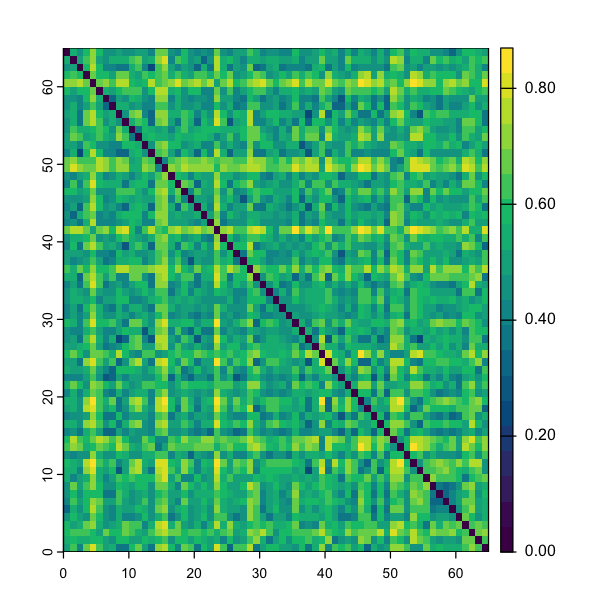
The first thing that jumps out is the diagonal - this is just that comparing a site to itself gives zero dissimilarity. All of the other pairwise combinations show a range of values.

If we want to compute the dissimilarity matrix based on another index, we can simply change method="bray" to any of the other indices provided in vegdist. Each dissimilarity metric has advantages and disadvantages but Bray-Curtis and Jaccard are commonly used for species abundance data.

Note that some of these indices in vegdist are not appropriate for abundance data. For example, Euclidean distance is widely used for environmental data (landscape metrics, geographic distance, temperature, altitude, etc) but is not ecologically meaningful for biodiversity data!

Principal coordinate analysis

We can now perform a principal coordinate analysis (PCoA) using the bray matrix as input. This is sometimes called classical multidimensional scaling, hence the function name: cmdscale. The PCoA will take your dissimilarity matrix and represent the structure in this dataset in a set of independent vectors (or ordination axes) to highlight main ecological trends and reduce noise. You can then use ordination axes to represent how similar (or dissimilar) two sites are with respect to the species they have.

Do not confuse classical multidimensional scaling with non-metric multidimensional scaling (NMDS), which is also very popular!

pcoa <- cmdscale(bray, k=8, eig=TRUE)

A PCoA calculates multiple independent axes of variation in the community dissimilarity. In fact, it calculates as many axes are there are sites. However, these different axes differ in how much variation they describe - we rarely want to consider more than a few. Here, we have only kept the data for the first eight (k=8). We are also hanging on the eigenvalues (eig=TRUE), which are measures of the amount variation associated with each axis.

Community separation in space

We will now explore community composition graphically, which is most convenient in two dimensions. We have to extract the new coordinates of the data before being able to plot them. Once again, it is wise to give clear names to each variable, otherwise we end up with variable names like X1.

# Extract the scores 
pcoa_axes <- pcoa$points
colnames(pcoa_axes) <- paste0('bray_raw_pcoa_', 1:8)

We can look at the correlations between all of those axes. We are using zapsmall to hide all correlations smaller than \(10^{-10}\) - as expected, none of these axes are correlated.

zapsmall(cor(pcoa_axes), digits=10)

A matrix: 8 × 8 of type dbl

	bray_raw_pcoa_1	bray_raw_pcoa_2	bray_raw_pcoa_3	bray_raw_pcoa_4	bray_raw_pcoa_5	bray_raw_pcoa_6	bray_raw_pcoa_7	bray_raw_pcoa_8
bray_raw_pcoa_1	1	0	0	0	0	0	0	0
bray_raw_pcoa_2	0	1	0	0	0	0	0	0
bray_raw_pcoa_3	0	0	1	0	0	0	0	0
bray_raw_pcoa_4	0	0	0	1	0	0	0	0
bray_raw_pcoa_5	0	0	0	0	1	0	0	0
bray_raw_pcoa_6	0	0	0	0	0	1	0	0
bray_raw_pcoa_7	0	0	0	0	0	0	1	0
bray_raw_pcoa_8	0	0	0	0	0	0	0	1

Now we can merge them onto the site data to make sure that the landscape and community metrics are matched by site.

# Convert the pcoa axis values to a data frame and label by site
pcoa_axes_df <- data.frame(pcoa_axes)
pcoa_axes_df$Site <- rownames(pcoa_axes)
# Merge onto the sites data - the PCoA axes get the labels X1 to X8
sites <- merge(sites, pcoa_axes_df, by='Site')

Now we can look to see how the community metrics reflect the landscape structure.

ggplot(sites, aes(bray_raw_pcoa_1, bray_raw_pcoa_2)) +
  geom_point(aes(colour = C600.pland)) + 
  scale_colour_gradientn(colors=hcl.colors(20)) + 
  theme_classic() 

Which patterns can you see from that plot? Along which axis do you see the trends varying the most, PCoA1 or PCoA2? Try looking at some of the other PCoA axes.

Exploring the data

Now plot PCoA axis 1 against the percentage of forest cover. Which trends do you get? And what about axis 2?

How many axes to consider

The eigenvalues show the variance - hence the information content - associated with each principal coordinate axis. Note that the eigenvalues are in descending order, so that the axes are numbered in order of their importance. Also note that some of the eigenvalues are negative - these axes cannot be interpreted biologically, but luckily this is never a problem for the first few axes which are the most meaningful anyway.

To make it easier to decide on how many dimensions we will keep, we look at the proportion of the total variance in the data set that is explained by each of the principal coordinates. The cumulative sum of eigenvalues describes how much of the variation in the original data is explained by the first n principal coordinates. We will drop the negative eigenvalues - they just confuse the cumulative calculation!

par(mfrow=c(1,2))
eig <- pcoa$eig[pcoa$eig >0] 
barplot(eig / sum(eig), main='Axis variation')
barplot(cumsum(eig)/ sum(eig), main='Cumulative variation')

# Print the percentage variation of the first 8 
head(sprintf('%0.2f%%', (eig / sum(eig)) * 100), n=8)

1. '21.16%'
2. '12.04%'
3. '8.85%'
4. '5.86%'
5. '4.92%'
6. '3.94%'
7. '3.68%'
8. '3.42%'

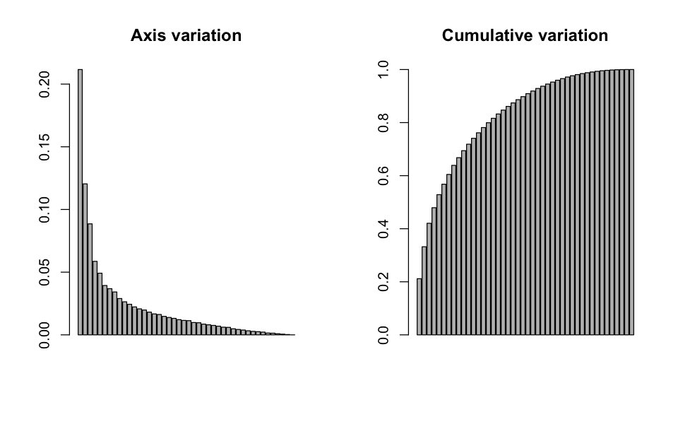
For this particular PCoA, the bar plot doesn’t really give a good indication about the number of principal coordinates axes to retain: the bars gradually decrease in size rather than showing a clear cutoff. From those plots, we can see that the first principal coordinate axis contains almost twice as much information as the second one (21.2% versus 12.0%). However, together they still only explain 33.2% of the variation.

However we shouldn’t blindly look at percentages. For instance, if one species in the matrix varies from 0 to 1,000 individuals - while all the other species vary from 0 to 10 - the percentage of information captured by the first axis will be considerably larger, but the axis will be only representing the variation in that particularly abundant species. If a scale function is applied to this hypothetical dataset, the percentage of information captured by the first axis will dramatically reduce, but this axis will provide more biologically meaningful results (i.e., it will better represent variation in the other species). Furthermore, the proportion of variation explained by the first axis reduces as -in this case- the number of species increases, so the amount of variation explained by the first axis is reasonable given that we have 140 species!

Explore the data - community metric variations.

All of the information from that PCoA depends entirely on our choices for the original dissimilarity matrix. If we change that metric then the positions of sites in the ordination space will change and so will the relative importances of the PCoA axes.

So, now explore varying the steps in this analysis. Change your inputs, change the dissimilarity metric and recalculate your ordination.

1. Use the command scaled_abundance <- scale(abundance) and use this as an input to vegdist. This will automatically scale the matrix by columns, so each column will have a mean of near 0, and standard deviation of 1.

2. Use presence-absence data by using the argument binary =TRUE with vegdist.

3. Try excluding the rare species (e.g. all species with 5 or less individuals):

   # choose columns (species) from abundance where total abundance is greater than 5
   total_abundance <- colSums(abundance)
   common <- abundance[,which(total_abundance > 5)]
   # data only has 71 columns now
   str(common)
   

4. Try using at least another dissimilarity metric.

Do any of these options seem to give a clearer relationship between the community composition and forest cover? There is no right or wrong answer here - different choices reflect different hypotheses.

Regression of landscape and community metrics

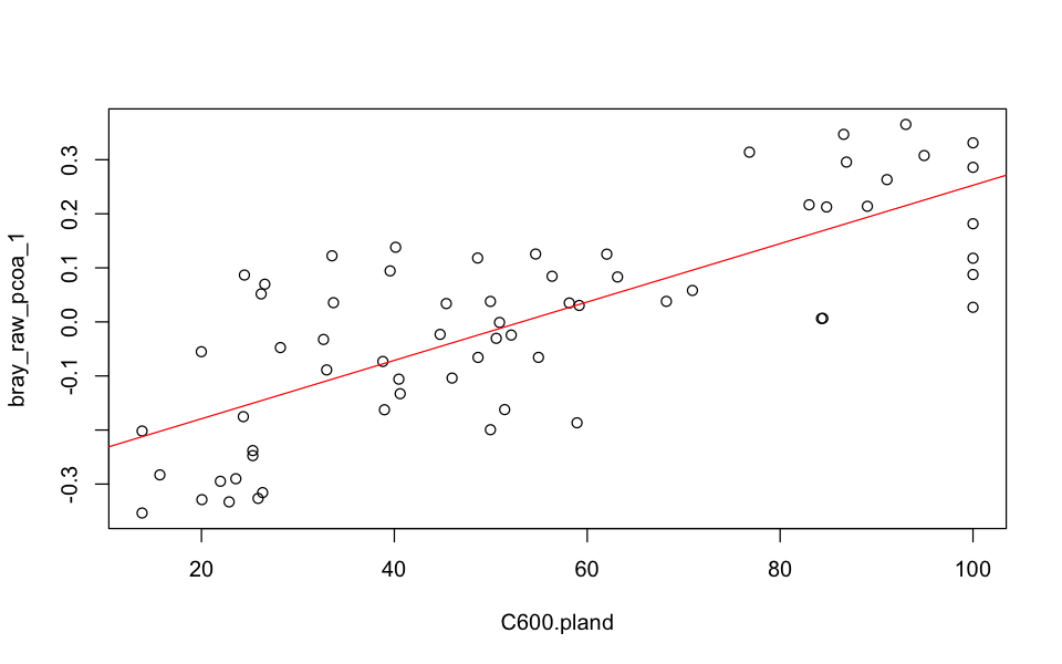
In addition to looking at correlations, we can fit linear models to predict how community composition varies between fragmented landscapes and continuous landscapes?

From the model below, forest cover at the 600m landscape scale explains 56.3% of the variation in community composition. Hence, we see that the first principal coordinate can reveal interesting biological trends, even if it only contained 21.2% of the information in the original data set (see above).

# Model community composition as a function of forest cover
mod_fc <- lm(bray_raw_pcoa_1 ~ C600.pland, data=sites)
summary(mod_fc)
# Plot the model
plot(bray_raw_pcoa_1 ~ C600.pland, data=sites)
abline(mod_fc, col='red')

Call:
lm(formula = bray_raw_pcoa_1 ~ C600.pland, data = sites)

Residuals:
      Min        1Q    Median        3Q       Max 
-0.225994 -0.087612  0.008098  0.078311  0.241801 

Coefficients:
              Estimate Std. Error t value Pr(>|t|)    
(Intercept) -0.2871733  0.0344031  -8.347 8.82e-12 ***
C600.pland   0.0054018  0.0005789   9.331 1.74e-13 ***
---
Signif. codes:  0 ‘***’ 0.001 ‘**’ 0.01 ‘*’ 0.05 ‘.’ 0.1 ‘ ’ 1

Residual standard error: 0.1239 on 63 degrees of freedom
Multiple R-squared:  0.5802,	Adjusted R-squared:  0.5735 
F-statistic: 87.06 on 1 and 63 DF,  p-value: 1.742e-13

Optional: Using R to assess functional diversity

The following section is an optional extra that shows how to use trait data to calculate functional diversity measures and incorporate those into landscape analyses. These techniques are not required for the group exercise but functional diversity is commonly used in landscape ecology and in broader diversity research.

Functional diversity

There are many measures of functional diversity, evenness and composition. Here we will only use one approach treedive, which is available in the vegan package. This calculates functional diversity as the total branch length of a trait dendrogram. The higher the number the more variation we have in traits within a community, which in theory correlates with a greater number of provided evosystem functions.

Petchey, O.L. and Gaston, K.J. 2006. Functional diversity: back to basics and looking forward. Ecology Letters 9, 741–758.

First, you will need to load the traits dataset, which includes information about:

• The main diet of all species, split into five categories (Invertebrates, Vertebrates, Fruits, Nectar, Seeds).

• The preferred foraging strata, split into four categories (Ground, Understory, Midstory, Canopy)

• The species’ mean body size (BMass).

• The number of habitats the species uses (Nhabitats), representing specialisation.

The values used for the diet and foraging strata are a semi-quantitative measure of use frequency: always (3), frequently (2), rarely (1), never (0). This matrix thus contains semi-quantitative variables and continuous variables.

traits <- read.csv("data/brazil/bird_traits.csv", stringsAsFactors = FALSE)
str(traits)

'data.frame':	140 obs. of  12 variables:
 $ Species      : chr  "species1" "species2" "species3" "species4" ...
 $ Invertebrates: int  1 1 1 3 3 3 2 3 2 3 ...
 $ Vertebrates  : int  0 0 0 0 0 0 2 0 2 0 ...
 $ Fruits       : int  0 0 0 0 0 0 1 0 1 1 ...
 $ Nectar       : int  3 3 3 0 0 0 0 0 0 0 ...
 $ Seeds        : int  0 0 0 0 0 0 0 0 0 0 ...
 $ Ground       : int  0 0 0 1 1 3 1 0 2 0 ...
 $ Understory   : int  3 1 2 3 1 1 2 3 2 3 ...
 $ Midstory     : int  1 2 2 1 3 0 2 1 2 1 ...
 $ Canopy       : int  1 2 2 0 0 0 2 0 0 0 ...
 $ BMass        : num  5 4.3 4.1 18.8 39 24.8 43.4 35.5 175 10.3 ...
 $ Nhabitats    : int  4 3 5 1 1 1 2 1 3 3 ...

That data needs to be restructured to name the data frame rows by species and remove the species names field to leave just the traits fields.

# Get a data frame holding only trait values, with rownames 
traits_only <- subset(traits, select=-Species)
rownames(traits_only) <- traits$Species

# Calculate the trait distance matrix
trait_dist <- taxa2dist(traits_only, varstep=TRUE)

# And get a trait dendrogram
trait_tree <- hclust(trait_dist, "aver")
plot(trait_tree, hang=-1, cex=0.3)

That dendrogram shows how species are clustered according to their trait similarity and the branch lengths measure an amount of functional diversity. The next step is to find the set of species in each site, reduce the dendrogram to just those species and find out the total branch length of that subtree.

trait_diversity <- treedive(abundance, trait_tree)

forced matching of 'tree' labels and 'comm' names

Now we just need to bring that data into our sites dataset to be able to use it.

trait_diversity <- data.frame(Site=names(trait_diversity),
                              trait_diversity=trait_diversity)
sites <- merge(sites, trait_diversity)

Final group exercise

Group exercise

Each group already have their landscape metrics measured, now you will need to focus on choosing one response variable that best represents variation in your data. Choose it carefully because you will need to defend your choice when you present your results.

• Groups SP01,04,08,13: Species richness or diversity

We have explored different ways to measure richness and diversity: select one of these
as your response variable.

• Groups 02,05,08,14: abundance or evenness

We have explored different ways to measure abundance and evenness: select one of these
as your response variable.

• Groups 03,06,09: community composition

We have explored different ways to do a community ordination. You can scale or not, use binary data or not, your choice. Select one of these approaches as your response variable.

Presenting your results on Friday

To present your results:

• Have one slide ready to present with the graph the relationship between your chosen response and explanatory variable.

• Ensure that the labels can be read on small screens!

• Include on this graph a fitted line, and ideally a confidence interval.

• Also include the \(r^2\) of the relationship and p-value.

Do not worry if you don’t find significant results! That’s to be expected. Each group will have a maximum of 5 minutes to present their results.

Two final notes on analyses:

1. Some of the variables we have used are better modelled using a GLM. That has not yet been covered in depth in the Masters modules. You are not expected to use a GLM here - although you can if you know how to use it and a GLM would be appropriate for your data.

2. Some explanatory variables will be correlated, so fitting more complex models (e.g. a multiple regression) may not be appropriate. This is the same problem of multicollinearity that was mentioned in the GIS species distribution modelling practical. For the moment, use single regressions for each explanatory variable at a time.